Additive Attention Mechanism

Attention mechanism is a very popular technique used in neural models today, with many powerful variations. Today, we will look at additive attention (Bahdanau et al., 2014), which was introduced as a solution to the fixed-sized hidden state problem of the seq2seq model.

Why attention?

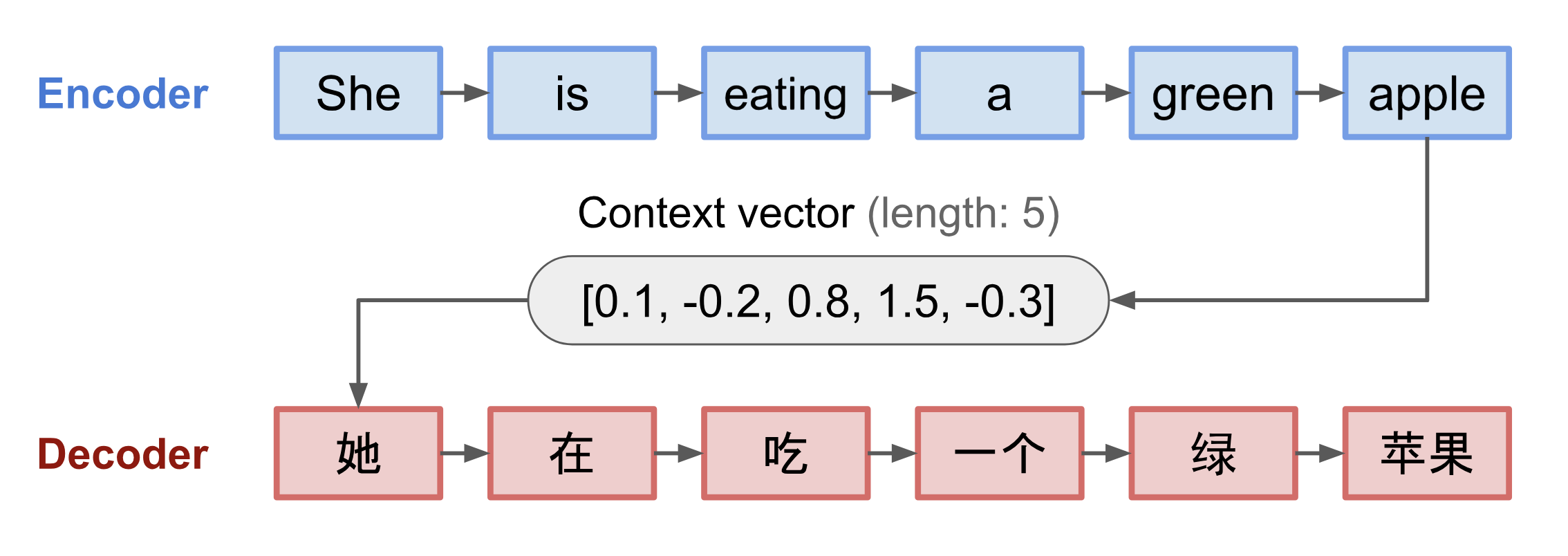
Source: (Weng, 2018)

In the motivating example of translating a sentence from one language to another, the sequence-to-sequence model featuring an encoder and decoder is commonly used. In the seq2seq model, the decoder takes in an input sequence and generates a context vector of pre-defined length. For purposes of illustration, one can interpret the context vector as the ‘meaning’ of the input sentence that is captured by the neural network. For the above example of translating from English to Chinese, the sentence “She is eating a green apple” comprising 6 words (tokens) is represented as a context vector of 5 numbers. This context vector is then used at the input of another network, the decoder, to generate the desired translated sentence in Chinese.

What are some potential problems of this method? The main failure mode for seq2seq models arises from when the input sequence is long. To quote the previous example, by the time last token in the sentence, “apple”, is fed into the encoder, the context vector (that has thus far encoded the first 5 words) would lose the representation for the first token “She”. When this context vector is subsequently fed into the decoder, the decoder is essentially forced to guess the first word in the source language, resulting in poor translations.

This arises from a known problem in training RNN-based models (the vanishing/exploding gradient problem), explained in further detail: To calculate the error between the network output and ground truth label during training, the gradients of each node across all time-steps are multiplied (a process known as backpropagation through time). When multiplying across many time-steps, small or large values of the gradients are compounded (imagine what happens when you take \(0.2\) to the \(10^{th}\) power), causing the gradients to converge at \(0\) or saturate at \(\infty\) and resulting in stalled training or NaNs (known as the vanishing and exploding gradient problem respectively). This failure mode in RNN-based encoder makes it hard for the model to properly encode for long-term dependencies between tokens many time-steps away (e.g. the first and last words in an input sentence), resulting in a context vector that represents the input sentence poorly.

Annotate, Align, Attend

The first improvement proposed in (Bahdanau et al., 2014) is using bidirectional RNN (BiRNN) as the encoder (Schuster and Paliwal, 1997). For each input sequence of length \(n\), the BiRNN reads the input sequence from the first to last token to generate the forward representation \(\overrightarrow{\boldsymbol{h}}_{j}\) for each token \(j\) in the sequence, and vice versa (last token to first token in reverse order) to form the backward representation \(\overleftarrow{\boldsymbol{h}}_{j}\). The two hidden states are then concatenated to form the an annotation for each word in the sequence \(\boldsymbol{h}_{j}\). The reason for generating a bidirectional representation for the sentence is to minimize effects of the vanishing gradient problem highlighted earlier. This is represented in the equation below:

\[\boldsymbol{h}_{j}=\left[\overrightarrow{\boldsymbol{h}}_{j}^{\top} ; \overleftarrow{\boldsymbol{h}}_{j}^{\top}\right]^{\top}, j=1, \ldots, n\]

Given the annotations obtained from the encoder, the decoder can now calculate the context vector \(\mathbf{c}_{i}\) for each token position \(i\), where \(i=1, \dots, m\) for output sequence length \(m\). The context vector is obtained by multiplying each annotation of the input sequence tokens with an alignment score \(\alpha_{i,j}\) as follows:

\[\mathbf{c}_{i}=\sum_{j=1}^{n} \alpha_{i,j} \boldsymbol{h}_{j}\]

\(\alpha_{i,j}\) is the alignment score, which determines how much each source hidden state should be considered for the output. It is calculated by adding the outputs of the decoder hidden state with the encoder outputs, after both are passed through separate linear layers (this is why the attention is termed as ‘additive’), followed by passing the output through a \(tanh\) activation layer. The weights of the aforementioned layers are parameterized and trained with the encoder-decoder model. Upon obtaining the context vector, we can then generate the decoder output as per normal seq2seq, by using the context vector and previous decoder time-step output as input into the decoder for each time-step.

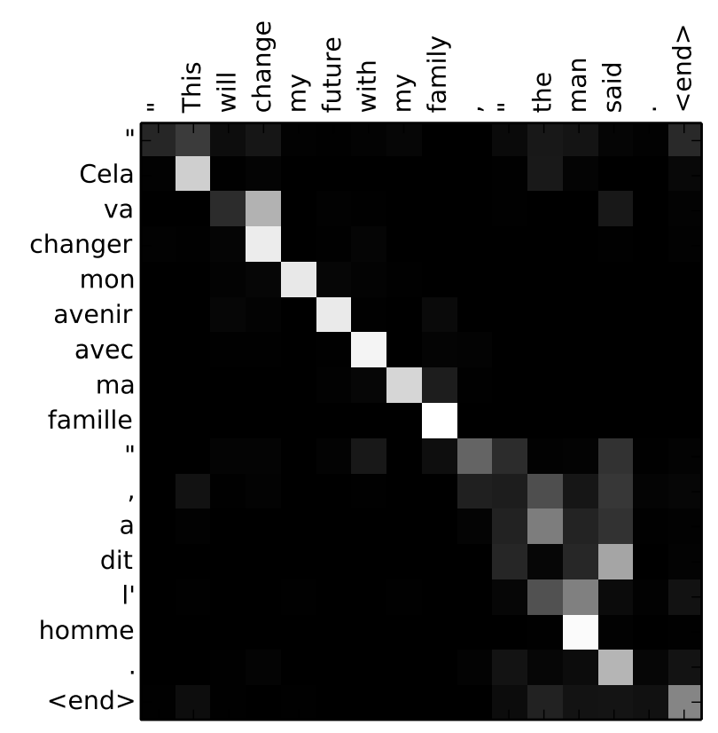
Source: (Bahdanau et al., 2014)

In essence, through learning the alignment scores, the model learns how much of the annotation vector in each encoder time-step it should use for different time-steps in the decoder. Intuitively, the decoder can be said to selectively focus on (pay attention to) different parts of the input sequence during output sequence generation. This visualized in the attention map above, which is a heatmap indicating the alignment scores between tokens in the source and target sentences (white indicated high alignment score). As the task is to translate an English sentence into French, an attention map with a highly activated diagonal is unsurprising given a similar Subject-Verb-Object order for both languages.